The world in pixels
Date:
March 2017 I took part in a spring school entitled
“Statistical Analysis of Hyperspectral and
High-Dimensional Remote-Sensing Data” organized by the
GIScience Group of the Friedrich-Schiller-University
Jena, March 13th–17th. The
spring school was an excellent place to learn more
about topics of remote sensing. It provided a large
overview on analysis of hyperspectral and multispectral
images through lectures, showcases and hands-on
exercises by specialists of the field. The
spring-school was dedicated to the (almost) exclusively
use of the R
language and environment with its
own libraries or as an interface with other open source
and free spatial tools (such as GDAL, QGIS, SAGA or
GRASS), similarly to this post.1
Hyperspectral?
Even if it sounds like the latest brand name for a new product2, the adjective hyperspectral qualifies the high density of information for each pixel in remote sensing imaging. This note try to explain briefly what it is it and starts with some basics on remote sensing.
Remote sensing: the basics
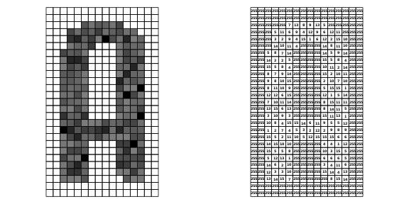
We can see photography as one of the oldest methods of remote sensing, in which the visible light (also called spectrum) of an object is stored on a medium (such as a film or a memory card). In the digital world, pixel (point) record a nuance of colour. For black-and-white images a value of grey is attributed to each pixel (point), often recorded between 0 (black) and 255 (white).
This figure presents the letter A at a very low resolution (i.e. with really large pixels, here 432 pixels), and decomposes it to understand how information may be recorded. The image on the left is the usual displayed form and the third image is a schematic representation, closer of how computer records the image. It uses 2 values of colour: 255 means white and 0 means black.
![]()
Obviously, to have the same letter A displayed in shades of grey, we only need to change the value of pixels with a value between 0 and 256 (256 or 28 is the length of a computer octet and is standard). The next figure represents the letter A with dark greys (left) and their numerical values (right). Note that I selected only low values of grey (i.e. dark greys) to better see the shape of the letter A without colours, using the perception difference between numbers with 1 or 2 digits vs the white value of 255.
Involving the spectrum
It is well know that “white” light is composed of colours. This is usually represented with the prism decomposing “white” light.
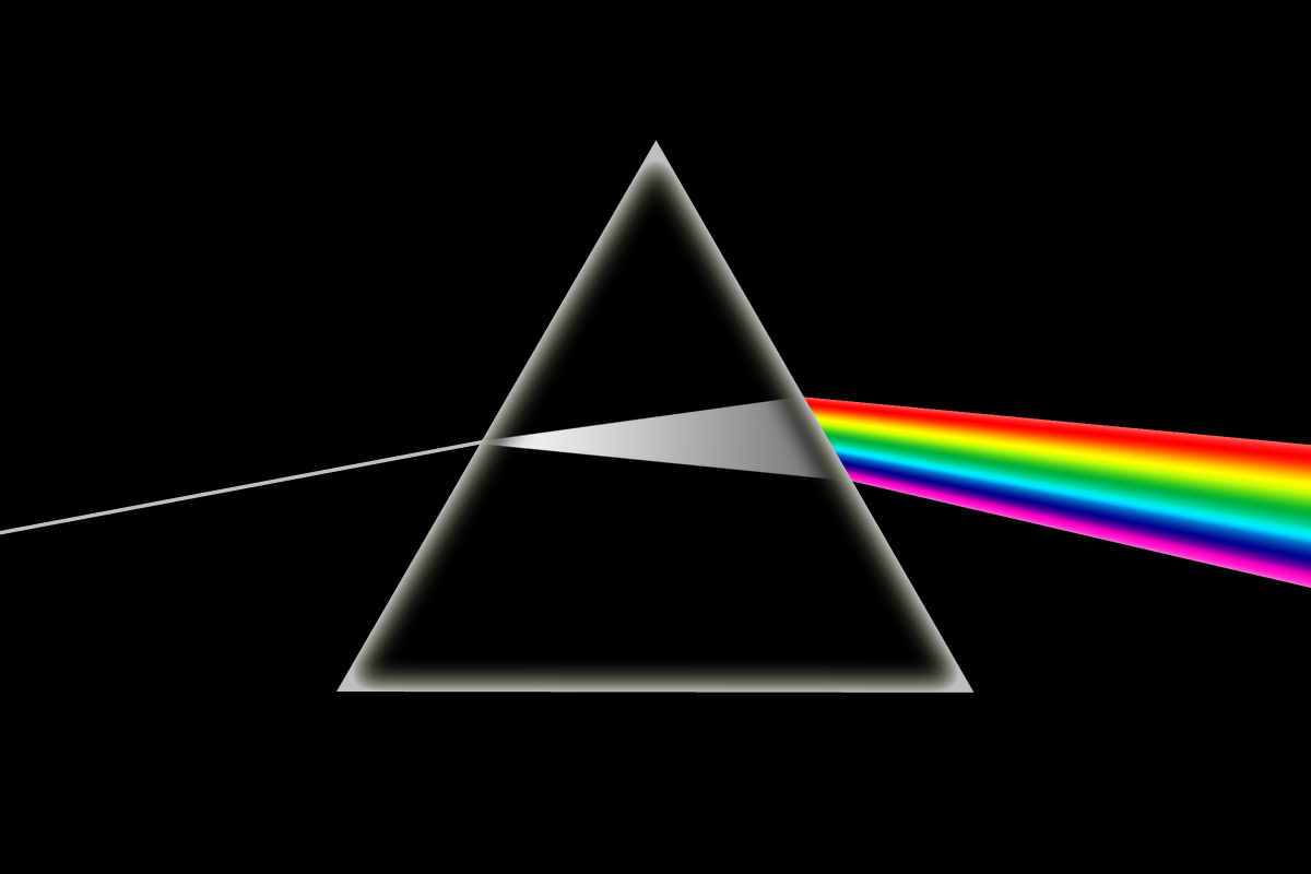
Optical dispersion effect observed when light passes through a prism, CC BY-SA Wikipedia (author: Vilisir)
The visible spectrum is the range of electromagnetic radiation perceived by humans. This radiation are defined by their wavelength (in Meter) and frequency (in Herz). Human eyes perceived radiations with a wavelength from about 380 to 750 nanometres.

Linear visible spectrum, CC BY-SA Wikipedia (author: Gringer)
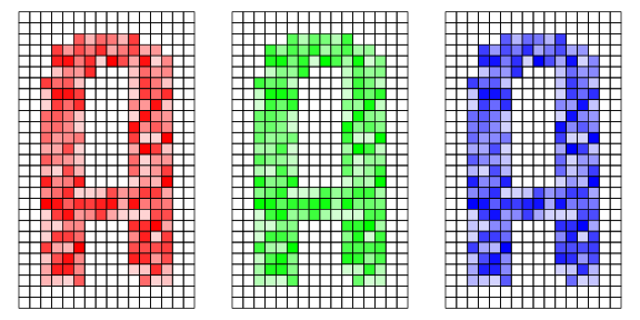
One of a typical way to record the visible light was to use three layer of values (red, green and blue) for each pixel using the propriety of these primary colours. This three colours can form all other colours by combining different proportion of them. If we have to imagine the letter A in colours, we could represent three grid like the black and white, one for each principal colour (red, green and blue), with a value between 0 and 255
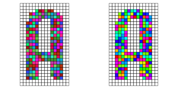
If we add the three layers we obtain colours, for example:
Multi and Hyperspectral
Now, the we have the basics, we can understand what are multispectral images and their difference with hyperspectral. We, human, see fine nuanced colours because our eyes, “our remote sensor” detect the entire visible range of wavelength. Sensors for remote sensing work only on specific wavelengths range, called “band”. This happens by choosing a range in which the sensor will record the reflectance. Multi-spectral sensors record several separate wavelength ranges, the colours are therefore different from what we see. On the other hand, sensors can record “non visible” wavelengths such as infra red, like in thermal camera recording or x-ray for radiograph sensing.
Multispectral sensors are the oldest kind of sensors that were used in satellites for remote sensing. These were sensoring only some bands of the reflectance, and were said to have a “low spectral resolution”. More recently multi-spectral sensors achieved a very high spectral resolution and have been called hyperspectral sensors. Instead of sensing a couple or a dozen of bands, they detect hundreds of very narrow bands on all the electronic spectrum, allowing a finer analyse and rendering of the data. Their advantage is a finer discrimination between difference, but the amount of data make there analysis more computational intensive. This is where the workshop started, to make sense of this kind of data, that are now becoming more and more available.
Acknowledgement
I would like to thanks the organizers of the workshops, the University of Jena granting a stipend covering the fees, ANAMED for covering the travel cost
License for the text of this post and the image (except for the MSCJ Life banner): CC BY-SA Néhémie Strupler
Notes
-
Code source for this post is available on my personal website nehemie.gitlab.io ↩
-
It reminds me Turkcell, a Turkish cell phone provider, that uses superlatives at every possible place to describe the speed of its products, such as “super”, “extra”, or even “turbo extra”, “ultra”… ↩