Yesterday’s post was about bike accidents by month. I was curious to see if the spatial repartition of accidents changes during the week and if there are some difference between working days and the weekend.
Exhibit of the day
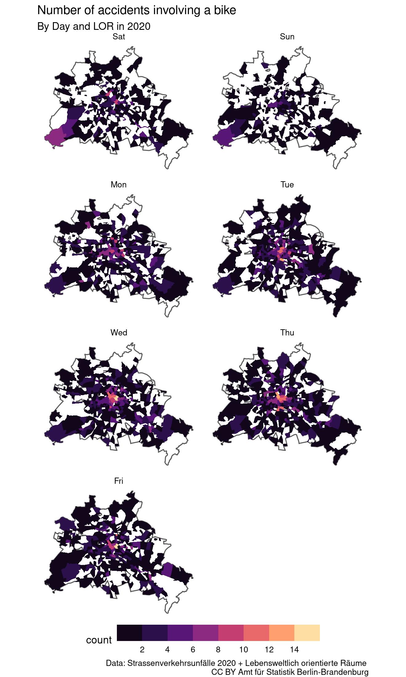
There are a some difference in the spatial repartition. In the southwest of Berlin, in the green lake area of Berlin, Wannsee and Nikolassee have more accidents the weekend than during the week and Sunday looks like the best day to cruise within the center of the city with a bike.
Show the code of the exhibit
library(sf)library(dplyr)library(ggplot2)crash <-read.csv2("raw_data/AfSBBB_BE_LOR_Strasse_Strassenverkehrsunfaelle_2020_Datensatz.csv",colClasses =c(rep("character", 3),rep("factor", 9),rep("integer", 6),rep("factor", 1),rep("numeric", 4)))colnames(crash) |>tolower() ->colnames(crash)crash[13:18] <-sapply(crash[13:18] , as.logical)crash$umonat <-factor(crash$umonat, levels =1:12)levels(crash$umonat) <-format(seq.Date(as.Date('2000-01-01'), by ='month', len =12), "%b")# Change name and reorder weekday# 1 = Sonntag 2 = Montag 3 = Dienstag# 4 = Mittwoch 5 = Donnerstag 6 = Freitag 7 = Samstaglevels(crash$uwochentag) <-format(seq.Date(as.Date('2000-01-02'), by ='day', len =7), "%a")crash$uwochentag <-factor(crash$uwochentag,levels(crash$uwochentag)[c(7,1:6)])crash <-subset(crash, istrad ==TRUE)crash |>group_by(lor_ab_2021, uwochentag) |>summarise(count =n()) -> crash_loredlor <-st_read("raw_data/lor_planungsraeume_2021.gml")colnames(lor)[1:6] |>tolower() ->colnames(lor)[1:6]lor$plr_id <- lor$plr_id |>as.factor()subset(lor, select=-bez) -> lorlor_outer <-st_as_sf(st_union(crash_sf))crash_sf <-full_join(lor, crash_lored, by=c(plr_id ="lor_ab_2021"))crash_sf <- crash_sf[!is.na(crash_sf$count), ]ggplot(crash_sf ) +geom_sf(data=lor_outer, fill="white") +geom_sf(aes(fill = count), colour ="transparent",show.legend =TRUE) +scale_fill_viridis_b(option ="A", n.breaks =10) +facet_wrap(vars(uwochentag), ncol =2) +theme_void() +theme(legend.key.width =unit(0.1, "npc"),legend.position="bottom") +labs(title ="Number of accidents involving a bike",subtitle ="By Day and LOR in 2020",caption ="Data: Strassenverkehrsunfälle 2020 + Lebensweltlich orientierte Räume \nCC BY Amt für Statistik Berlin-Brandenburg")ggsave("2022-03-11_bike_crash_day_lor.jpg", width=6.0,height=10, bg="white", dpi =220)
Berlin’s map of bike accident by weekday and LOR. Data: Strassenverkehrsunfälle nach Unfallort in Berlin 2020 + Lebensweltlich orientierte Räume − CC BY Amt für Statistik Berlin-Brandenburg>